Boundary Performance#
Testing the performance of the CPML allows for building optimal models. The maximum spatial step and source frequency should be accounted for when setting up the domain to reduce numerical instability. There are 3 primary parameters - \(\kappa\), \(\sigma\), and \(\alpha\) - that affect the absorption and attenuation of wave energy as it travels into and out of the boundary.
:math:`kappa` is the scaling factor that adjust the effective speed of the wave within the CPML. \(\kappa\) enhances absorption by compressesing the wave field and increasing the path length. A higher \(\kappa_{\text{max}}\) value leads to better absorption by compressing the fields more, but values that are too high can cause numerical instability. Lower values improve stability but at the cost of less effective boundaries. In the model domain, \(\kappa\) is 1 then increases to its maximum value as distance into the CPML increases. An optimal maximum value is given by:
however theory and practice sometimes diverge given the problem. When this happens, tuning the value involves a more heuristic approach.
\(\sigma\) represents the electrical conductivity within the CPML which introduces a loss term that attenuates the wave. This is the main damping mechanism in the CPML. Higher \(\sigma_{\text{max}}\) values will increase damping however, excessively high values can cause rapid change in the wave field and numerical instability. The optimal sigma value can be computed using
followed by a scaling factor, \(\rho\), to find the maximum value
\(\alpha\) is an artificial loss parameter that add an additional loss term to stabilize the CPML. This is primarily effective in eliminating evancescent and grazing waves with higher max values enhancing the dampening effect. Typically, a small non-zero value is used, and while there are a few equations for computing an optimum \(\alpha_{\text{max}}\), it was found that
provides a generalized term for numerical stability and optimal performance.
There are different approaches to estimating the reflected power. This script computes the cumulative energy density in the boundary region over the full time interval by using a grid search over varying the proportionality constant, \(\rho\), and \(\kappa_{\text{max}}\) values. Relative to a reference value, we can gauge the performance of the boundary conditions. The parameters can be adjusted by the user to optimize them. They are defined in the prjrun module and consist of: kappa_max, sig_opt_scalar, alpha_max_scalar, Rcoef, NP, and NPA. The reflection coefficient, Rcoef, is specific to seismic CPML, and NP and NPA are the exponential terms for grading the CPML from the inner boundary to the outer boundary max value. *NPA is specific for calculating \(\alpha\) since it is auxiliary to both \(\sigma\) and \(\kappa\). If changing these parameters is desired, you can do so by importing the prjrun module and directly assigning the variables: For instance,
from seidart.routines import prjrun

prjrun.kappa_max = 7e-1
prjrun.NP = 4
prjrun.NPA = 3
prjrun.kappa_max = 1.1e0
prjrun.sig_opt_scalar = 0.8
prjrun.alpha_max_scalar = 1.1e0
The defualt values are:
alpha_max_scalar = 1.0
kappa_max = 5
sig_opt_scalar = 1.2
*Rcoef* = 0.0010
*NP* = 2
*NPA* = 2
A breakdown of the code is as follows.
Import the appropriate modules.
import numpy as np
from glob2 import glob
import seaborn as sns

from seidart.routines import prjrun, sourcefunction
from seidart.routines.definitions import *


prjfile = 'em_boundary_performance.prj'
domain, material, __, em = prjrun.domain_initialization(prjfile)
Define the range of the variables that we want to use in the estimate.
dk = 0.1
ki = 1.0
kf = 15
kappa_max = np.arange(ki, kf+dk, dk)

sk = 0.05
si = 0.1
sf = 10.0
sig_opt_scalar = np.arange(si,sf+sk, sk)

source_frequency = np.array([
        2.0e7
])

ref_kappa = 1.0
ref_sigma = 1.0

m = len(kappa_max)
n = len(sig_opt_scalar)
p = len(source_frequency)
Prep the model and pre-allocate variables.
cumulative_power_density_x = np.zeros([m,n,p])
cumulative_power_density_z = np.zeros([m,n,p])
datx = np.zeros([domain.nx + 2 * domain.cpml, domain.nz + 2*domain.cpml])
datz = datx.copy()

# Load the project and get going
prjrun.status_check(
        em, material, domain, prjfile, append_to_prjfile = True
)
timevec, fx, fy, fz, srcfn = sourcefunction(em, 10, 'gaus1')
- Loop through each value and
Overwrite the current values for kappa_max and sig_opt_scalar
Run the model
Zero out the model domain within the boundaries in order to easily sum the energy.
Re the domain dimensions to their original values.
for ii in range(m):
        prjrun.kappa_max = kappa_max[ii]
        for jj in range(n):
                prjrun.sig_opt_scalar = sig_opt_scalar[jj]
                for kk in range(p):
                        print( f"{ii}/{m-1} - {jj}/{n-1} - {kk}/{p-1}" )
                        # Zero out the
                        datx[:,:] = 0.0
                        datz[:,:] = 0.0
                        em.f0 = source_frequency[kk]
                        prjrun.runelectromag(
                                em, material, domain
                        )
                        domain.nx = domain.nx + 2*domain.cpml
                        domain.nz = domain.nz + 2*domain.cpml

                        fnx = glob('Ex.*.dat')
                        fnz = glob('Ez.*.dat')
                        for filex, filez in zip(fnx, fnz):
                                datx += ( read_dat(
                                        filex, 'Ex', domain, is_complex = False, single = True
                                ) )**2
                                datz += ( read_dat(
                                        filez, 'Ez', domain, is_complex = False, single = True
                                ) )**2

                        datx[domain.cpml:-(domain.cpml+1),domain.cpml:-(domain.cpml+1)] = 0.0
                        datz[domain.cpml:-(domain.cpml+1),domain.cpml:-(domain.cpml+1)] = 0.0

                        cumulative_power_density_x[ii,jj,kk] = datx.sum()
                        cumulative_power_density_z[ii,jj,kk] = datz.sum()

                        # Typically the domain dimensions are changed and stored in an Array
                        # object, but in this case we have to manually change them so that
                        # an error isn't returned in runelectromag or read_dat
                        domain.nx = domain.nx - 2*domain.cpml
                        domain.nz = domain.nz - 2*domain.cpml
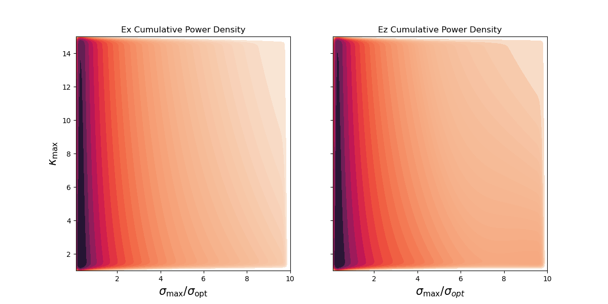
Visualize the output using a bivariate KDE plot. Other types of plotting exists, but this is a quick and commonly used method.
# This is setup to compute many different source frequencies.
cpd_x = cumulative_power_density_x[:,:,0]
cpd_z = cumulative_power_density_z[:,:,0]

# Create the kde plots
sigma_grid, kappa_grid = np.meshgrid( sig_opt_scalar, kappa_max)
kappa_flat = kappa_grid.ravel()
sigma_flat = sigma_grid.ravel()
cpd_x_flat = cpd_x.ravel()
cpd_z_flat = cpd_z.ravel()

fig, axs = plt.subplots(1,2, figsize = (12,6), sharey = True)
sns.kdeplot(x = sigma_flat, y = kappa_flat, weights = cpd_x_flat/cpd_x_flat.max(), fill = True, ax = axs[0], cmap = "rocket_r", bw_adjust = 0.25, levels = 30)
sns.kdeplot(x = sigma_flat, y = kappa_flat, weights = cpd_z_flat/cpd_x_flat.max(), fill = True, ax = axs[1], cmap = "rocket_r", bw_adjust = 0.25, levels = 30)

axs[0].set_ylabel(r'$\kappa_{\text{max}}$', fontsize = 16)
axs[0].set_xlabel(r'$\sigma_{\text{max}}/\sigma_{\text{opt}}$', fontsize = 16)
axs[0].set_title('Ex Cumulative Power Density')
axs[0].set_xlim( sig_opt_scalar.min(), sig_opt_scalar.max() )
axs[0].set_ylim( kappa_max.min(), kappa_max.max() )
axs[1].set_ylabel(r'$\kappa_{\text{max}}$', fontsize = 16)
axs[1].set_xlabel(r'$\sigma_{\text{max}}/\sigma_{opt}$', fontsize = 16)
axs[1].set_title('Ez Cumulative Power Density')
axs[1].set_xlim( sig_opt_scalar.min(), sig_opt_scalar.max())
axs[1].set_ylim(kappa_max.min(), kappa_max.max() )
plt.show()
Save the outputs. This takes a while to run for even a small model. We can also run different ranges of alpha or sigma in batches and concatenate the data sets later.
The figure generated can be seen below. A high \(\kappa_{\text{max}}\) along with a high \(\rho\) would intuitively be less numerically stable than low values for each. What we see is that in the high value of each, not much energy is penetrating the boundary and instead being reflected back into the domain. However, at the opposite end of the spectrum, we want to make sure that energy isn’t passing through the boundary layer. We can conclude that`kappa_{text{max}}` and \(\rho\) values around 1.0-3.0 and 0.5-1.0, respectively, would be good choices and consistent with the litterature. Our estimate for kappa_{text{max}} was virtually 1.0 which implies that there is no difference between \(\kappa\) within and outside of the boundary.